Vibrating string equation (without damping)

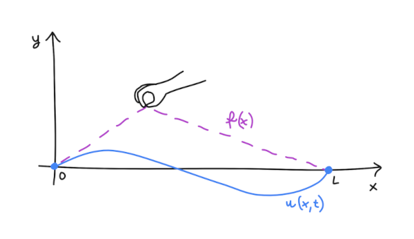
Vibrating string without damping is represented by the following differential equation:

$$ \begin{cases} \begin{array}{l@{\ }l@{\ }l} \frac{{{\partial ^2}u}}{{\partial {t^2}}} = {a^2}\frac{{{\partial ^2}u}}{{\partial {x^2}}} , & \hspace{0.25in} 0 \leqslant x \leqslant L , 0 \leqslant t \leqslant \infty , & \hspace{0.25in} \text{string equation} ; \\ u\left( {0,t} \right) = u\left( {L,t} \right) = 0 , & \hspace{0.25in} 0 \leqslant t \leqslant \infty , & \hspace{0.25in} \text{boundary conditions} ; \\ u\left( {x,0} \right) = f\left( x \right) , \frac{{\partial u}}{{\partial t}}\left( {x,0} \right) = 0 , & \hspace{0.25in} 0 \leqslant x \leqslant L , & \hspace{0.25in} \text{initial conditions}; \end{array} \end{cases} \tag{1} $$

Splitting the string equation into two coupled equations

We need to transform the equation:

$$ \frac{{{\partial ^2}u}}{{\partial {t^2}}} = {a^2}\frac{{{\partial ^2}u}}{{\partial {x^2}}} \tag{2} $$

Let's introduce E value, which represents time derivative of the y-position:

$$ E = \frac{{{\partial}u}}{{\partial {t}}} \tag{3} $$

So now, we've got two coupled equations:

$$ \begin{cases} \begin{array}{l@{\ }l@{\ }l} \frac{{{\partial}E}}{{\partial {t}}} = {a^2}\frac{{{\partial ^2}u}}{{\partial {x^2}}} \\ \frac{{{\partial}u}}{{\partial {t}}} = E \end{array} \end{cases} \tag{4} $$

We will use them in the numerical solution.

Eulerian mesh

Current state of the vibrating string we will store in an 1-dimentional differential Eulerian mesh. We will store there finite number of points of the string and for each point its current y-position (u) and its time derivative of the y-position (E), which is in fact the current velocity of the particular point of the string.

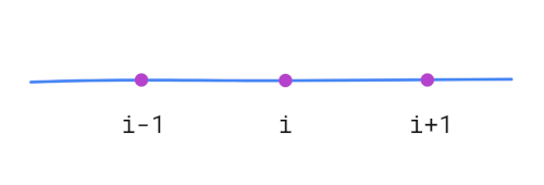
To implement it, we just need to create two 1-dimensional arrays: U and E. Lenght of both arrays is the same and represents number of points of the string. Number of points is up to us. More points - more accurate calculations, but cost of calculations bigger.

Numerical solution

In numerical solution we will calculate state of the string (u and E) for the next time-step (time n+1) basing on current state of the string (time n).

Numerical solution for the cupled equations (4) looks like this:

$$ \begin{cases} \begin{array}{l@{\ }l@{\ }l} E^{n+1}_{i} = E^{n}_{i} + {a^2} \frac{ u^{n}_{i+1} - 2 u^{n}_{i} + u^{n}_{i-1} }{ \Delta x^{2} } \Delta t \\ u^{n+1}_{i} = u^{n}_{i} + E^{n+1}_{i} \Delta t \end{array} \end{cases} \tag{5} $$

In the first equation there was used the second-order central difference approximation. In the second - linear dependence.

In code of the simulation this fragment looks like this:

  _calculateNextStep () {
    let currentE = this.eulerianMesh['e'];
    let currentU = this.eulerianMesh['u'];
    let nextE = [];
    let nextU = [];

    // Apply boundary conditions
    nextE[0] = 0;
    nextE[this.pointsNumb - 1] = 0;
    nextU[0] = 0;
    nextU[this.pointsNumb - 1] = 0;

    // Calculations for other points
    for (let i = 1; i < (this.pointsNumb - 1); i++) {
      nextE[i] = currentE[i] + Math.pow(this.v, 2) * ((currentU[i+1] - 2*currentU[i] + currentU[i-1]) / Math.pow(this.deltaX, 2)) * this.deltaT;
    }
    for (let i = 1; i < (this.pointsNumb - 1); i++) {
      nextU[i] = currentU[i] + nextE[i] * this.deltaT;
    }

    this.eulerianMesh = {
      'e': nextE,
      'u': nextU,
    };
  }

Initial conditions

As an initial state of the Eulerian mesh we have to set:

• u: y-positions of the points for the initial shape of the string
• E: fill with zeros, because velocity of each point of the string equals zero before we release tensioned string

Simulation

You can play with the simulation here or by clicking the image below:

You can compare bahavior of the string from the simulation with the real experiment: YouTube: Motion of Plucked String

GitHub

Code of the simulation is available on GitHub here https://github.com/tomdwor/vibrating-string

References

• Markowe Wykłady z Matematyki: równania różniczkowe, Marek Zakrzewski, GiS 2020
• Symulacje komputerowe w fizyce, Maciej Matyka, Helion 2021